Learning with DVRF - Step 11 - Part 2 - Let's get that GDB running

Step 11 - “Hello” GDB demonstrated in 5 parts

In the previous post, we were able to get the appropriate “pre-checks” done for GDB/pwndbg. We trudged through the steps necessary to get GDB/pwndbg correctly aligned with steps to get a better debugging experience. This post will briefly examine the “hello” binary in GDB/pwndbg and then go through each line step-by-step in GDB/pwndbg. This is blog post 11, part 2 of 5, of post x in the learning with DVRF project series.

Part 2: What do all of these symbols mean?

1. In pwndbg, type in:
   
   c
   
   
   
   
2. Here we can see no warnings, we’re getting stack information from objects outside of our binary (e.g. uClibc), accurate backtrace information with stack information from external libraries (e.g. uClibc), and things look to be better since we now have more accurate representations of information.
   
3. Now we can debug all the things! Actually, at this point, we are going to get the same results as when we did this manually in a previous blog post. The main (no, not the function, hah!) object of this post was to get more familiarity with GDB/pwndbg (such as start/stopping GDB, hooking up binaries, setting/removing/checking breakpoints), making sure we broke on the actual entry point of main, and getting our symbols from external libraries loaded appropriately.
   
4. There are some subtle differences though from when we disassembled this by “hand” within objdump and doing this interactively within GDB/pwngdb. We will step through “hello” with GDB/pwndbg to observe how the stack and registers fluctuate with each step.
   
5. Let’s review the four panes in GDB/pwndbg:
   
   
   
   
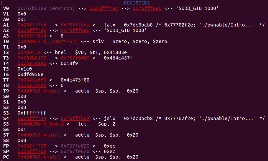
6. In the first “pane” labeled “Registers” we can see the MIPS registers and how they’re used within our program. This is pretty much a way better view of the registers than relying upon “i r / info registers” with the default view that GDB provides.
   
   pwndbg registers:
   
   
   
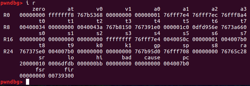
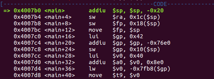
   GDB’s default view of registers:
   
   
   
7. The second pane of “Code” is the MIPS assembly of the code being executed. This looks fairly similar to the disassembled output from objdump. However, we see that instead of seeing the values in decimal (e.g. in the first line) we get a more consistent view of numbers and see hex representation of the number being manipulated.
   
   
   
8. The third pane of “Stack” represents a view of the stack as it changes through the execution of the program.
   
   
   
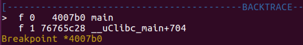
9. The fourth pane of “Backtrace” represents the caller functions which shows how the program got to where it is now.